I don’t understand how so many people have so many weird ideas about timescale. I think it stems from some simulators not allowing modules to have a timescale declaration if it already parsed modules without one. So, for example, if you have module1 without a timescale and module2 with a timescale, and you then compile module1 followed by module2, you get an error. If you compile module2 followed by module1, then all is well, and module1 just uses the timescale from module2. Now, I agree that this is weird. There should just be a default timescale that applies at the beginning of the simulation. Let’s look at some examples that I have seen that attempt to overcome this problem.

The Special-Timescale-File-Goes-First Method

In this solution, everyone agrees that the very first file the compiler ever sees is a special timescale file with only a default timescale directive. I suppose that this solution is an attempt to enforce the way all the tools should probably work. The problem with this approach is that it relies on everyone to use the same simulation tool flow. In some environments this can be possible, but I’ve seen this approach backfire when bringing up a new tool or flow, or even when just changing the rules in a makefile.

The Include-a-Special-File Method

In this scheme, everyone agrees to include a special timescale file with a default timescale– unless they need their own custom timescale declaration. This approach removes the requirement that any particular file needs to go first. However, it now builds a special requirement of your flow into the RTL. This leads to portability issues if you move the RTL into another flow.

The Correct Method– always specify a timescale

I think that the correct approach is to specify a timescale before the first module in every source file which contains a module. Use this method even (and I want to make this absolutely clear) if you don’t make any reference to time in the module. Using this technique, your file will always be correct. If it is, then first, it will declare some timescale for everyone else. If not, then no harm done. And if some further module specifies time without specifying a timescale, then there’s some fault with that module.

Of course, it’s possible to use this method in combination with the first if you have some code that can’t be changed, and thus can’t have a timescale added. The include file approach is just wrong-headed. I don’t know why it would ever be a good idea– especially if your module actually cares about what the timescale is.

Many designers think that recursive techniques cannot be applied to hardware design. I’m not really sure where this misconception comes from. While it is true that in Verilog ’95 you could not use recursion because the language did not support it, with Verilog 2001, recursion is possible. Recursion is really useful for describing hardware that has a tree structure. Let’s use a priority encoder as an example.

A priority encoder takes as input a bit vector and produces the bit number of the highest (or lowest) bit set and also an indication that some input bit was set. For example with an 8-bit encoder and an input of ‘b00101110, the output would be 5 because bit number 5 is the highest bit set.

The base case

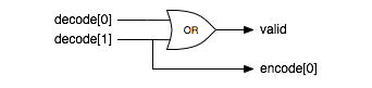
For a 2-bit input, a priority encoder is pretty simple. The valid output is just the OR of the two input bits. The bit number output is just the higher input bit. In schematics it looks something like this.

A 2-bit priority encoder

The recursive case

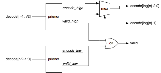
For an encoder which is 2ⁿ-bits wide, we could join two 2^n-1 bit wide priority encoders together like this.

Recursive implementation of a priority encoder

Verilog code

So what does the code for this look like? It’s pretty simple. If the input vector is two bits wide, then we just implement the base case. Otherwise, if the width is not a power of two, then we pad out the input with zero bits to the next power of two width and then instantiate a power of two width encoder. If the width is a power of two, then we build the encoder out of two encoders half the size.

module priencr #(parameter width = 64)
  (
   input [width-1:0] decode,
   output [log2(width)-1:0] encode,
   output valid
   );

  function [31:0] log2;
    input reg [31:0] value;
    begin
      value = value-1;
      for (log2=0; value>0; log2=log2+1)
	value = value>>1;
    end
  endfunction

  generate
    if (width == 2)
      begin
	assign valid = |decode;
	assign encode = decode[1];
      end
    else if (width & (width-1))
      priencr #(1<<log2(width)) priencr ({1<<log2(width) {1'b0}} | decode,
                                         encode,valid);
    else
      begin
	wire [log2(width)-2:0] encode_low;
	wire [log2(width)-2:0] encode_high;
	wire valid_low, valid_high;
	priencr #(width>>1) low(decode[(width>>1)-1:0],encode_low,valid_low);
	priencr #(width>>1) high(decode[width-1:width>>1],encode_high,valid_high);
	assign valid = valid_low | valid_high;
	assign encode = valid_high ? {1'b1,encode_high} : {1'b0,encode_low};
      end
  endgenerate
endmodule

Wrap up

The only gotchas with recursion are vendor support. I have come across vendors who don’t think recursion is possible in Verilog 2001 because the standard doesn’t say it is specifically supported. The Verilog 2005 standard is very clear that recursion is allowed to help with this problem.

Recursion can be a very powerful way to express tree-like structures in hardware.